ENGR5003 Lecture 13 worked example 2 (slides 11-14)
A gas-turbine power plant operating on an ideal Brayton cycle (Figure 1) has a pressure ratio of 8. The gas temperature is 300 K at the compressor inlet and 1300 K at the turbine inlet. Calculate the gas temperatures at the exits of the compressor and the turbine. Also calculate the back work ratio, the cycle work and the thermal efficiency.
Use the ideal-gas air table (Cengel Table A-17), where is the relative pressure, with for an isentropic process:
| T (K) | h (kJ/kg) | |
|---|---|---|
| 300 | 300.19 | 1.386 |
| 540 | 544.35 | 11.10 |
| 760 | 778.18 | 39.27 |
| 780 | 800.03 | 43.35 |
| 1300 | 1395.95 | 330.9 |
Then repeat with the cold-air-standard assumptions (, ) and compare.
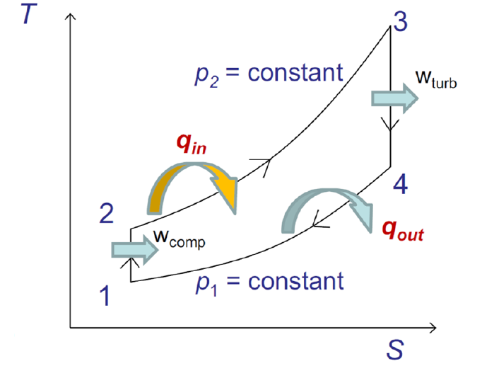
Formulas you may need
- SFEE, adiabatic, negligible KE and PE: (on the formula sheet)
- Isentropic relation with relative pressure: (learn this, Lecture 13; tables provided)
- Back work ratio , (on the formula sheet)
- Brayton efficiency (constant ): (on the formula sheet)
- Linear interpolation (learn this)
- (a)Temperatures at the compressor and turbine exits (air tables).
- (b)Back work ratio, net (cycle) work and thermal efficiency (air tables).
- (c)The same quantities with constant specific heats (cold-air standard).