ENGR201 2023 A2 (ENGR5001)

ENGR201 2023 A2Past paperOld spec ENGR201First25 marks30 min

ENGR201 Engineering Analysis 2023 Section A, A2[VALID] official answers

Consider the RL circuit shown in Figure A2. $i_1$ and $i_2$ are the currents in each loop, which satisfy the differential equations

$L_1\frac{di_1}{dt} + R_2(i_1 - i_2) + R_1 i_1 = v(t) \qquad \text{(A3a)}$ $L_2\frac{di_2}{dt} + R_2(i_2 - i_1) = 0 \qquad \text{(A3b)}$

Assume $L_1 = 0.8$ H, $L_2 = 1$ H, $R_1 = 1.4\ \Omega$ , $R_2 = 1\ \Omega$ and $v(t) = 100$ V for $t > 0$ . The initial conditions are $i_1(0) = 0$ and $i_2(0) = 0$ .

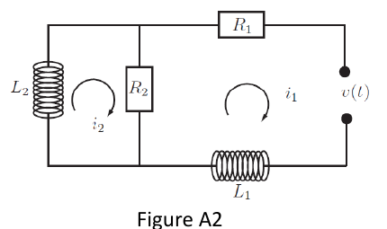Figure A2: two-loop circuit; loop 1 (current i1) contains v(t), R1, L1 and the shared R2; loop 2 (current i2) contains R2 and L2.

Formulas you may need

$\mathcal{L}\left[\dfrac{di}{dt}\right] = sI(s) - i(0)$ ; constant $100 \to \dfrac{100}{s}$ (learn this; printed in the ENGR201 Laplace table)
$e^{at} \leftrightarrow \dfrac{1}{s - a}$ (learn this; printed in the ENGR201 Laplace table)
Cover-up rule for distinct poles: residue at $s = p$ is $\left[(s - p)F(s)\right]_{s = p}$ (learn this)
Final value theorem $\lim_{t \to \infty} i(t) = \lim_{s \to 0} sI(s)$ (learn this)

(a)
Find the Laplace transforms of the currents.
[10]2:1
(b)
Find the currents by the inverse Laplace transform.
i1 at t = 1 s =A
i2 at t = 1 s =A
[12]
(c)
Explain what happens to the currents when $t$ increases.
i1 = i2 as t -> infinity =A
[3]2:2